Introduction to the precision-recall plot

The precision-recall plot is a model-wide measure for evaluating binary classifiers and closely related to the ROC plot. We’ll cover the basic concept and several important aspects of the precision-recall plot through this page.

For those who are not familiar with the basic measures derived from the confusion matrix or the basic concept of model-wide evaluation, we recommend reading the following two pages.

For those who are not familiar with the basic concept of the ROC plot, we also recommend reading the following page.

Introduction to the ROC (Receiver Operating Characteristics) plot

If you want to dive into making nice precision-recall plots right away, have a look at the tools page:

Tools for ROC and precision-recall

Precision-recall shows pairs of recall and precision values

The precision-recall plot is a model-wide evaluation measure that is based on two basic evaluation measures – recall and precision. Recall is a performance measure of the whole positive part of a dataset, whereas precision is a performance measure of positive predictions.

Four ovals respectively represent observed labels, four outcomes, recall, and precision. — A dataset has two labels (P and N), and a classifier separates the dataset into four outcomes – TP, TN, FP, FN. The precision-recall plot is based on two basic measures – recall and precision that are calculated from the four outcomes.

The precision-recall plot uses recall on the x-axis and precision on the y-axis. Recall is identical with sensitivity, and precision is identical with positive predictive value.

A naïve way to calculate a precision-recall curve by connecting precision-recall points

A precision-recall point is a point with a pair of x and y values in the precision-recall space where x is recall and y is precision. A precision-recall curve is created by connecting all precision-recall points of a classifier. Two adjacent precision-recall points can be connected by a straight line.

An example of making a precision-recall curve

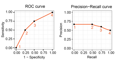
We’ll show a simple example to make a precision-recall curve by connecting several precision-recall points. Let us assume that we have calculated recall and precision values from multiple confusion matrices for four different threshold values.

Threshold	Recall	Precision
1	0.0	0.75
2	0.25	0.25
3	0.625	0.625
4	1.0	0.5

We first added four points that matches with the pairs of recall and precision values and then connected the points to create a precision-recall curve.

A Precision-Recall curve and four Precision-Recall points. — The plot shows a precision-recall curve connecting four precision-recall points.

3 important aspects of making an accurate precision-recall curve

Unlike the ROC plot, it is less straight-forward to calculate accurate precision-recall curves since the following three aspects need to be considered.

Estimating the first point from the second point
- AUC cannot be calculated without the first point
Non-linear interpolation between two points
- curves with linear interpolation tend to be inaccurate for small datasets, imbalanced datasets, and datasets with many tied scores
Calculating the end point
- the end point should not be extended to the top right (1.0, 1.0) nor the bottom right (1.0, 0.0) except in the case that observed labels are either all positives or all negatives

We’ll show an example of these aspect by creating a precision-recall curve.

An example of recall and precision pairs

We use four pairs of recall and precision values that are calculated from four threshold values.

Point	Threshold	Recall	Precision
1	1	0	–
2	2	0.5	0.667
3	3	0.75	0.6
4	4	1	0.5

We explain the three aspects by using the three pairs of consecutive points.

Points 1-2: estimating the first point
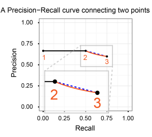
Points 2-3: non-linear interpolation
Points 3-4: calculating the end point

Points 1-2: Estimating the first point from the second point

The first point should be estimated from the second point because the precision value is undefined when the number of positive predictions is 0. This undefined result is easily explained by the equation of precision as PREC = TP / (FP + TP) where (FP + TP) is the number of positive predictions.

There are two cases of estimating the first point depending on the true positives of the second point.

The number of true positives (TP) of the second point is 0
The number of true positives (TP) of the second point is not 0

Case 1: TP is 0

Since the second point is (0.0, 0.0) for this case, it is easy to estimate the first point, which is also (0.0, 0.0). In other words, the first point is not necessary to be estimated for this case.

Case 2: TP is not 0

This is also the case for our example, and the second point is (0.5, 0.667). We can estimate the first point by drawing a horizontal line from the second point to the y-axis. Hence, the first point is estimated as (0.0, 0.667).

First two Precision-Recall points. — Drawing a horizontal line from the second position to the y-axis to estimate the first point.

Points 2-3: Non-linear interpolation between two points

Davis and Goadrich proposed the non-linear interpolation method of precision-recall points in their article (Davis2006). The equation described in their article is

$\mathrm{y = \displaystyle \cfrac{TP_A + x}{TP_A + x + FP_A + \cfrac{FP_B - FP_A}{TP_B - TP_A} \cdot x}}$

where y is precision and x can be any value between 0 and |TP_B – TP_A|. A smooth curves can be created by calculating many intermediate points between two points A and B.

Non-linear interpolation of two Precision-Recall plots. — Two precision-recall points are connected by non-linearly. The blue dot line shows a straight line between points 2 and 3, whereas the red solid curve shows the correct non-linear interpolation between them.

An intermediate point 2.5 for points 2-3

Let us assume the second point has 2 TPs and 1 FP and the third point has 3 TPs and 2 FPs.

Point 2: (0.5, 0.667)
Point 3: (0.75, 0.6)

	Point 2	Point 3
TP (# of true positives)	2	3
FP (# of false positives)	1	2
Recall	0.5	0.75
Precision	0.667	0.6

We then define the intermediate point 2.5 as the middle point where recall is 0.625. We show that the precision value of point 2.5 can be different for linear and non-linear interpolation.

Linear interpolation

Since point 2.5 is the center point of the second and the third points, the precision value is 0.633.

Point 2.5: (0.625, 0.633)

Non-linear interpolation

We calculate the precision value by

$\mathrm{\displaystyle \cfrac{TP_{point2} + x}{TP_{point2} + x + FP_{point2} + \cfrac{FP_{point3} - FP_{point2}}{TP_{point3} - TP_{point2}} \cdot x}}$

with the following values.

TP_point2: 2
FP_point2: 1
TP_point3: 3
FP_point3: 2
x: 0.5

The calculated precision value is 0.625.

Point 2.5: (0.625, 0.625)

Points 3-4: Calculating the end point

The end point of the precision-recall curve is always (P / (P + N), 1.0). For instance, the end point is (0.5, 1.0) from (4 / (4 + 4), 1.0) when P is 4, and N is 4. Subsequently, the end position and the previous position should be connected by non-linear interpolation.

The end point of a Precision-Recall curve. — The end point is precision curve can be calculated as P / (P + N). It is 0.5 when P is 4 and N is 4.

Interpretation of precision-recall curves

Similar to a ROC curve, it is easy to interpret a precision-recall curve. We use several examples to explain how to interpret precision-recall curves.

A precision-recall curve of a random classifier

A classifier with the random performance level shows a horizontal line as P / (P + N). This line separates the precision-recall space into two areas. The separated area above the line is the area of good performance levels. The other area below the line is the area of poor performance.

Two Precision-Recall curves of random classifiers for different positive and negative ratio. — A random classifier shows a straight line as P / (P + N). For instance, the line is y = 0.5 when the ratio of positives and negatives is 1:1, whereas 0.25 when the ratio is 1:3.

A precision-recall curve of a perfect classifier

A classifier with the perfect performance level shows a combination of two straight lines – from the top left corner (0.0, 1.0) to the top right corner (1.0, 1.0) and further down to the end point (1.0, P / (P + N)).

Two Precision-Recall curves of perfect classifiers for different positive and negative ratio. — A perfect classifier shows a combination of two straight lines. The end point depends on the ratio of positives and negatives. For instance, the end point is (1.0, 0.5) when the ratio of positives and negatives is 1:1, whereas (1.0, 0.25) when the ratio is 1:3.

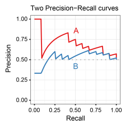
Precision-recall curves for multiple models

It is easy to compare several classifiers in the precision-recall plot. Curves close to the perfect precision-recall curve have a better performance level than the ones closes to the baseline. In other words, a curve above the other curve has a better performance level.

Two Precision-Recall curves for two classifiers A and B - The plot indicates classifier A outperforms classifier B. — Two precision-recall curves represent the performance levels of two classifiers A and B. Classifier A clearly outperforms classifier B in this example.

Noisy curves for small recall values

A precision-recall curve can be noisy (a zigzag curve frequently going up and down) for small recall values. Therefore, precision-recall curves tend to cross each other much more frequently than ROC curves especially for small recall values. Comparisons with multiple classifiers can be difficult if the curves are too noisy.

AUC (Area Under the precision-recall Curve) score

Similar to ROC curves, the AUC (the area under the precision-recall curve) score can be used as a single performance measure for precision-recall curves. As the name indicates, it is an area under the curve calculated in the precision-recall space. An approximate but easy way to calculate the AUC score is using the trapezoidal rule, which is adding up all trapezoids under the curve.

The AUC score can be calculated by the trapezoidal rule. — The areas of the three trapezoids 1, 2, 3 are 0.335, 0.15875, and 0.1375. The AUC score is then 0.63125.

Although the theoretical range of AUC score is between 0 and 1, the actual scores of meaningful classifiers are greater than P / (P + N), which is the AUC score of a random classifier.

Four Precision-Recall curves with their AUC scores. — The score is 1.0 for the classifier with the perfect performance level (P) and 0.5 for the classifier with the random performance level (R). The plot clearly shows classifier A outperforms classifier B, which is also supported by their AUC scores (0.7 and 0.52).

One-to-one relationship between ROC and precision-recall points

Davis and Goadrich introduced the one-to-one relationship between ROC and precision-recall points in their article (Davis2006). In principle, one point in the ROC space always has a corresponding point in the precision-recall space, and vice versa. This relationship is also closely related with the non-linear interpolation of two precision-recall points

A ROC curve and a precision-recall curve should indicate the same performance level for a classifier. Nevertheless, they usually appear to be different, and even interpretation can be different.

In addition, the AUC scores are different between ROC and precision-recall for the same classifier.

Difference of the AUC scores between ROC and Precision-Recall. — ROC shows the same AUC score for A (0.61) and B (0.61), but precision-recall shows different scores for A (0.62) and B (0.53).

3 important characteristics of the precision-recall plot

Among several known characteristics of the precision-recall plot, three of them are important to consider for accurate the precision-recall analysis.

Interpolation between two precision-recall points is non-linear.
The ratio of positives and negatives defines the baseline.
A ROC point and a precision-recall point always have a one-to-one relationship.

These characters are also important when the plot is applied to imbalanced datasets. For more details about the precision-recall plot with imbalanced datasets, we recommend reading the following pages.

25 thoughts on “Introduction to the precision-recall plot”

Omar Colombo Mendoza says:

September 14, 2016 at 11:38 am

Hi!

I don’t understand if endpoint needs to be calculated or if it is just taken from the observations. In case it has to be calculated, I don’t understand how to do that (why P and N are equal 4).

I would appreciate if you could clarify my doubts.
Thanks in advance.

LikeLike

Reply
1. takaya says:
  
  September 14, 2016 at 11:43 pm
  
  Hi!
  
  Yes, the end point always needs to be calculated. It represents the case where all data instances are predicted as positive (you can see the section “Confusion matrix for TH=0.0” on the Basic concept of model-wide evaluation page for an example).
  
  Our test set here has 8 instances with 4 positives (P=4) and 4 negatives (N=4). True positive is 4 (TP=4), and the number of instances as predicted as positive is 8 when the all data instances are predicted as positive, which is the case for the end point. Therefore, TP is always equivalent with P at the end point. You can simply calculate the precision at the endpoint as TP / (# of predicted as positive) = P / (# of all data instances) = P / (P + N).
  
  I hope this will help.
  
  LikeLiked by 2 people
  
  Reply
  1. Alex says:
    
    May 3, 2017 at 4:30 am
    
    Hi, the end point is well recall is 1 which indicates all labels positive are correctly predicted. But there can be more than one threshold that meets this condition. How do we determine the precision in this case?
    
    LikeLike
  2. takaya says:
    
    May 10, 2017 at 1:27 am
    
    Hi Alex,
    
    Precision is always calculated as TP / (# of predicted as positive), and it is common to have multiple precision values for one recall value. It is drawn as a vertical line in that case. This also applies when recall is 1.
    
    LikeLike
Tong Shu Li says:

December 9, 2016 at 1:35 am

Hi Takaya,

I believe the location of the random classifier line in the Precision-Recall plot is incorrect in figures 5b and 6b (the figures associated with sections “A Precision-Recall curve of a random classifier” and “A Precision-Recall curve of a perfect classifier”).

The ratio of positives to negatives is stated as 3:1. By the given formula of P/(P+N), this should give 0.75 instead of 0.25 as shown. A simpler fix would be to state that the P:N ratio as 1:3 instead of 3:1.

Cheers,
Toby

LikeLike

Reply
1. takaya says:
  
  December 9, 2016 at 3:27 am
  
  Hi Toby,
  
  Yes, the correct P:N ratio should be 1:3 instead of 3:1 as suggested. My bad! I have fixed both figures and uploaded them. Thanks a lot. I appreciate your help.
  
  Cheers,
  Takaya
  
  LikeLike
  
  Reply
Arpan Shrivastava says:

April 11, 2017 at 3:02 pm

Hi Takaya,

I have some queries about precision-recall curve,
1. Can we use this curve to determine THRESHOLD value for classification as we do by using ROC curve (basically balancing recall and specificity ).
2. Are these two thresholds necessarily different?
3.If my problem statement is like that precision is more important than recall or overall accuracy ,should i use threshold determined by precision-recall caurve?

Thanks in advance. 🙂

LikeLike

Reply
1. takaya says:
  
  April 17, 2017 at 3:02 am
  
  Hello Arpan,
  
  It’s a good question. There are many methods that can be used to find the optimal threshold value, but it is usually quite difficult find one that works on all unseen data (your independent test datasets, for instance).
  
  For ROC:
  * The balance point where sensitivity = specificity.
  * The closest point to (0, 1).
  * Yonden’s J statistics: You can calculate max(sensitivity + specificity) instead.
  
  Different methods usually achieve different threshold values. The main problem here is that your positive predictions tend to have way too many false positives if you use any of these threshold values on imbalanced data sets. You can use them as long as your datasets are balanced. There are alternative methods that can take error cost weights, but the optimal error costs are usually unknown so that you don’t know how to specify the weights.
  
  For precision-recall:
  * Break-even point: the point where precision = recall.
  * max(F-score): F-score is a harmonic mean of precision and recall.
  
  You can use them to find the optimal threshold value, but I strongly suggest you test the value on your validation and test datasets. It should work fine even for imbalanced datasets.
  
  Regards,
  Takaya
  
  LikeLike
  
  Reply
Pingback: Introduction to the precision-recall plot – computerCalledVarun()
Pingback: What is true positive and true negative – confusion matrix | Vikas D More
Matt says:

October 1, 2017 at 5:01 am

I believe this is a small typo. Shouldn’t the part near the end read: (1.0, P / (P + FN))
?

“A classifier with the perfect performance level shows a combination of two straight lines – from the top left corner (0.0, 1.0) to the top right corner (1.0, 1.0) and further down to the end point (1.0, P / (P + N)).”

LikeLike

Reply
1. takaya says:
  
  October 12, 2017 at 7:34 pm
  
  The end point can be always calculated as (1, P / (P + N)) since TP and FP become equivalent to P and N when all instances are predicted as positives.
  
  In other words, the precision can be calculated as TP / (TP + FP) = P / (P + N) at the end point.
  
  LikeLike
  
  Reply
  1. Pinglin says:
    
    July 18, 2018 at 7:13 pm
    
    Hi takaya,
    
    Can you kindly explain how come FP will become equivalent to TN at the end point? I failed to get the point that TN can ever play a role in Precision-Recall Curve. Thank you.
    
    LikeLike
  2. takaya says:
    
    July 18, 2018 at 7:27 pm
    
    Hi,
    
    The number of FPs is not equivalent with the number of TNs but with N (the number of all instances labeled as negative in your test set) at the end point. TN is not considered in precision-recall curves, as you said.
    
    Hope this helps.
    
    LikeLike
  3. Pinglin says:
    
    July 19, 2018 at 5:28 am
    
    Hi,
    
    But in that case, the classifier is no longer a “perfect” classifier, right? It is nothing but a naive classifier classifying all instances as positive at recall=1.0.
    
    I had an impression that a perfect classifier is to have precision=1.0 and recall=1.0.
    
    LikeLike
  4. takaya says:
    
    July 19, 2018 at 7:16 pm
    
    The precision-recall plot evaluates a model/classifier with varying multiple threshold values. The perfect classifier above means that there is one threshold that makes it to produce perfect predictions. Its precision-recall curve passes (1, 1) as recall = 1 and precision = 1 in that case. It does not produce perfect predictions if you use a threshold value at the end point.
    
    LikeLike
Pingback: Operating Thresholds: Behind the Scenes | The Official Blog of BigML.com
Pingback: Operating Thresholds: Behind the Scenes | Premium Blog! | Development code, Android, Ios anh Tranning IT
Martinbop says:

May 6, 2018 at 11:31 pm

Hellow my name is Martinbop. Wery good-hearted article! Thx 🙂

LikeLike

Reply
VIyer says:

July 16, 2019 at 5:31 pm

Great article that gives clarity on the subject

LikeLike

Reply
Pingback: Krzywa Precision-Recall jak ją wykreślić i zinterpretować - About Data
Prageeth says:

May 23, 2020 at 12:06 am

Hi, can a Precision-recall curve can be started from (0,0)? I’m getting such a PR curve for my baseline model. Would you be able to explain it? Thank you!

LikeLike

Reply
1. takaya says:
  
  May 25, 2020 at 2:26 pm
  
  Yes, precision can be any value in [0, 1] or undefined when recall is 0.
  
  Example:
  Assume we have 4 instances and pick up 0.7 as a threshold for positive prediction.
  
  Scores: 0.8, 0.6, 0.3, 0.2
  Labels: N, P, N, P
  Predicted: P, N, N, N
  
  Then, the confusion matrix would be as follows.
  
  FP=1 TP=0
  TN=1 FN=2
  
  From the matrix:
  TPR(recall) = TP / (TP + FN) = 0 / (0 + 2) = 0.0
  PPV(precision) = TP / (TP + FP) = 0 / (0 + 1) = 0.0
  
  LikeLike
  
  Reply
Filipa says:

November 26, 2020 at 7:48 pm

Thank you so much for your article, I was getting precision recall curves that don’t start at (0,1) and assuming they were wrong because of it.
Could you please mention any bibliography you might have used when composing this article?

Thanks again
Filipa

LikeLike

Reply
1. takaya says:
  
  November 27, 2020 at 12:39 am
  
  We used our own tool called precrec. It’s a CRAN package.
  
  LikeLike
  
  Reply