
We introduce basic performance measures derived from the confusion matrix through this page. The confusion matrix is a two by two table that contains four outcomes produced by a binary classifier. Various measures, such as error-rate, accuracy, specificity, sensitivity, and precision, are derived from the confusion matrix. Moreover, several advanced measures, such as ROC and precision-recall, are based on them.
After studying the basic performance measures, don’t forget to read our introduction to precision-recall plots (link) and the section on tools (link). Also take note of the issues with ROC curves and why in such cases precision-recall plots are a better choice (link).
Test datasets for binary classifier
A binary classifier produces output with two class values or labels, such as Yes/No and 1/0, for given input data. The class of interest is usually denoted as “positive” and the other as “negative”.

Test dataset for evaluation
A dataset used for performance evaluation is called a test dataset. It should contain the correct labels (observed labels) for all data instances. These observed labels are used to compare with the predicted labels for performance evaluation after classification.

Predictions on test datasets
The predicted labels will be exactly the same if the performance of a binary classifier is perfect, but it is uncommon to be able to develop a perfect binary classifier that is practical for various conditions.

Hence, the predicted labels usually match with part of the observed labels.

Confusion matrix from the four outcomes
A confusion matrix is formed from the four outcomes produced as a result of binary classification.
Four outcomes of classification
A binary classifier predicts all data instances of a test dataset as either positive or negative. This classification (or prediction) produces four outcomes – true positive, true negative, false positive and false negative.
- True positive (TP): correct positive prediction
- False positive (FP): incorrect positive prediction
- True negative (TN): correct negative prediction
- False negative (FN): incorrect negative prediction

Confusion matrix
A confusion matrix of binary classification is a two by two table formed by counting of the number of the four outcomes of a binary classifier. We usually denote them as TP, FP, TN, and FN instead of “the number of true positives”, and so on.
| Predicted | |||
| Positive | Negative | ||
| Observed | Positive | TP (# of TPs) | FN (# of FNs) |
| Negative | FP (# of FPs) | TN (# of TNs) |
Basic measures derived from the confusion matrix
Various measures can be derived from a confusion matrix.
First two basic measures from the confusion matrix
Error rate (ERR) and accuracy (ACC) are the most common and intuitive measures derived from the confusion matrix.
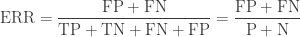
Error rate
Error rate (ERR) is calculated as the number of all incorrect predictions divided by the total number of the dataset. The best error rate is 0.0, whereas the worst is 1.0.

Accuracy
Accuracy (ACC) is calculated as the number of all correct predictions divided by the total number of the dataset. The best accuracy is 1.0, whereas the worst is 0.0. It can also be calculated by 1 – ERR.


Other basic measures from the confusion matrix
Error costs of positives and negatives are usually different. For instance, one wants to avoid false negatives more than false positives or vice versa. Other basic measures, such as sensitivity and specificity, are more informative than accuracy and error rate in such cases.
Sensitivity (Recall or True positive rate)
Sensitivity (SN) is calculated as the number of correct positive predictions divided by the total number of positives. It is also called recall (REC) or true positive rate (TPR). The best sensitivity is 1.0, whereas the worst is 0.0.


Specificity (True negative rate)
Specificity (SP) is calculated as the number of correct negative predictions divided by the total number of negatives. It is also called true negative rate (TNR). The best specificity is 1.0, whereas the worst is 0.0.


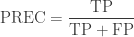
Precision (Positive predictive value)
Precision (PREC) is calculated as the number of correct positive predictions divided by the total number of positive predictions. It is also called positive predictive value (PPV). The best precision is 1.0, whereas the worst is 0.0.

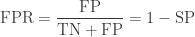
False positive rate
False positive rate (FPR) is calculated as the number of incorrect positive predictions divided by the total number of negatives. The best false positive rate is 0.0 whereas the worst is 1.0. It can also be calculated as 1 – specificity.

Correlation coefficient and F-score
Mathews correlation coefficient and F-score can be useful, but they are less frequently used than the other basic measures.
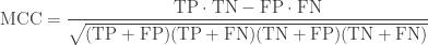
Matthews correlation coefficient
Matthews correlation coefficient (MCC) is a correlation coefficient calculated using all four values in the confusion matrix.
F-score
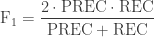
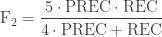
F-score is a harmonic mean of precision and recall.

β is commonly 0.5, 1, or 2.

An example of evaluation measure calculations
Let us assume that the outcome of some classification results in 6 TPs, 4 FNs, 8 TNs, and 2 FPs.

First, a confusion matrix is formed from the outcomes.
| Predicted | |||
| Positive | Negative | ||
| Observed | Positive | 6 | 4 |
| Negative | 2 | 8 |
Then, the calculations of basic measures are straightforward once the confusion matrix is created.
| measure | calculated value | |
|---|---|---|
| Error rate | ERR | 6 / 20 = 0.3 |
| Accuracy | ACC | 14 / 20 = 0.7 |
| Sensitivity True positive rate Recall |
SN TPR REC |
6 / 10 = 0.6 |
| Specificity True negative rate |
SP TNR |
8 / 10 = 0.8 |
| Precision Positive predictive value |
PREC PPV |
6 / 8 =0.75 |
| False positive rate | FPR | 2 / 10 = 0.2 |
Other evaluation measures
Please see the following pages for more advanced evaluation measures.

well explained.
LikeLike
It’s a relief to find soneome who can explain things so well
LikeLike
Excellent explanation..great understanding…
LikeLike
The explanation and the examples are very nice….
LikeLike
Very nice illustration and explanation.
LikeLike
Very precise, simple yet clear description and any one can easily understand and remember it. Thanks for the wonder full post.
LikeLike
“False positive rate (FPR) is calculated as the number of incorrect negative predictions… ” Should not be: incorrect positive predictions?
LikeLike
Oops. I just corrected it. Thank you very much for your help!
LikeLike
very nice explanation.Thank u so much
LikeLike
Great explanation, everything makes sense now!! Thank you!
LikeLike
very smooth explanation. i have a small question. for multiple classes, how am i going to calculate the error rate. according to this, i calculate the class.error for each classes but the general “OOB estimate of error rate” is different from what the algorithm calculates. What could have been the thing I miss? Many thanks
LikeLike
The calculation of the error rate is still the same even for multi-class classifications as: (# of misclassified instances) / (# of total instances). Some of machine learning methods that use bootstrap resampling require no validation datasets during training because they can use OOB instead. For instance, you can calculate an error rate for each subsample, and then you can aggregate all of them to calculate the mean error rate. You still need a test data set to evaluate your final model, though.
LikeLike
Very Very good explanation. Thank you
LikeLike
When evaluating these values, are there acceptable values that we can say it’s good/bad?
LikeLike
No, not really. You need to consider other factors, such as your problem domain, test data sets and so on, to estimate whether the performance of your model is good or bad from these metrics. But, you can always use them for comparisons among multiple models and hypotheses.
LikeLike
Good and Clear explanation.
LikeLike
A.A
Sir! i am using Weka tool and run DecisionTable classifier model and get confusion Matrix but i need to Label as a TP,TN,FP and FN
a b Class
2781 0 a = No
26 425 b = Yes
So, please help me sirr
Regards
LikeLike
Assume that the labels Yes (b) and No (a) respectively represent positive and negative, and the matrix is as follows:
a . b . <– predicted/classified labels
2781 . 0 . (a = No in your test set)
26 . 425 . (b = Yes in your test set)
Then, TPs = 425, TNs = 2781, FPs = 0 and FNs = 26.
LikeLike
A lot of thanks takaya…..
Regards
Ibrar
LikeLike
Excellent explanation and most of the research papers do not cover many of these parameters
LikeLike
Very nice explanation.
I have a question, Shouldn’t Precision (Positive Predictive Value) be 60% i.e. 6(TP)/6(TP)+4(FP)=0.6.
Thanks in advance.
LikeLike
The number of FPs is not 4 but 2 in the example above. So, precision is 0.75 as 6 / (6 + 2).
LikeLiked by 2 people
Absolutely wonderful explanation.
LikeLike
Amazing explanation with crystal clear concepts.
LikeLike
Excellent
LikeLike
Excellent explanation and most article do not cover many of these parameters
LikeLike
Well explained. Thanks for sharing.
LikeLike
Good, but FN and FP have set interchange.
LikeLike
Was a bit confused at first with the concepts but after reading this I now understand it, it’s very well explained. Thank you!
LikeLike